Theoretical method and application of dynamic consolidation range of high fill earth and stone
-
摘要: 强夯法在高填方加固中广泛应用,而基于理论计算的加固范围确定方法很少,且对于描述横向加固宽度的方法更少,而加固深度和宽度是进行强夯设计的关键。基于此,建立了基于随机介质理论的强夯内部沉降计算方法,模型仅含有影响角β和压缩系数η两个参数;通过承德机场土石料强夯现场试验表明,该模型能很好地计算土体内部沉降量;同时,提出了临界沉降量的概念,并确定出无黏性土石料的临界沉降量为0.04 m;最后,结合临界沉降量给出了基于夯坑深度的强夯加固范围的快速查图结果。实现了强夯加固理论方法的创新和快速推广应用,为相关工程提供直接参照结果。Abstract: The dynamic compaction method is widely used in high fill reinforcement, but there are few methods to determine the reinforcement range based on the theoretical calculation, furthermore, there are fewer methods to describe the transverse reinforcement width. However, the reinforcement depth and width are the key to the dynamic compaction design. On this basis, the method for calculating the internal settlement of dynamic compaction based on the random medium theory is established. The model only contains two parameters, i.e., the influence angle β and the compression coefficient η. The field tests on dynamic compaction of earth and stone in Chengde Airport shows that the model can be used to calculate the internal settlement of soils. The concept of the critical settlement is put forward, and the critical settlement of cohesionless earth rock materials is determined to be 0.04 m. Finally, the fast chart results of dynamic consolidation range based on the depth of ramming pit are given. The proposed method realizes the innovation and rapid application of dynamic consolidation theory and method, and provides direct reference results for the related projects.
-
Keywords:
- dynamic compaction /
- internal settlement /
- reinforcement range /
- random medium /
- chart checking
-
0. 引言
土–水特征曲线(SWCC)描述了土体含水率随基质吸力变化的函数关系,在非饱和土的研究中起着非常重要的作用。以SWCC为理论基础,非饱和土在强度、渗透、固结和本构关系等方面的研究已在过去的几十年里得到了广泛的开展[1-3]。SWCC相关数据可以通过压力板法、滤纸法和蒸气平衡等方法进行测量[4-5]。然而,这些方法仅能获得离散的数据点,还需将试验数据与相关模型进行拟合并形成明确的函数表达式才能直接应用于其他理论研究。
SWCC模型可划分为物理模型和经验模型。前者主要是基于域理论、土壤参数或孔隙几何特征所建立的模型,后者一般是采用统计分析方法通过拟合建立的模型,其拟合参数大都不具备物理意义。因此,物理模型相较于经验模型能更准确地解释土体性质。另一方面,现有经验模型[6-7]通常假设土体为理想的孔隙空间结构,即假设土体具备单峰特征。然而,已有研究表明,许多土壤的孔隙结构表现出双峰特征[8-9],因此,这些经验模型更符合单峰孔隙结构土,对于具备双峰孔径分布特征的土体并不适用。
双峰SWCC模型通常由两种方法建立。第一种是将单峰SWCC模型进行叠加[10-11],该方法得到的双峰SWCC模型通常为经验模型,存在较多没有明确物理意义的拟合参数。第二种是根据土体的结构特征,如双峰粒径/孔径分布特征等建立模型。Liu等[12]利用对数正态分布近似土体的孔径分布函数,基于此建立了双峰SWCC模型。Satyanaga等[13]基于双峰粒径分布的数学表达式建立了双峰SWCC模型。这类模型中的参数具有一定物理意义,但其表达式通常较为复杂。
大量研究表明,在自然条件下,许多类型的岩土体具有符合分形特征的孔径和粒径分布,有学者已证明分形理论能较为有效地描述岩土体颗粒和孔隙分布规律,基于此,现已形成较为成熟的土-水特征曲线分形模型体系,其有效性已得到较为充分的验证[14-19]。目前,土体分形特征的研究主要面向单峰孔隙结构土,对双峰孔隙结构土的工程特性研究相对较少。
本研究通过叠加土体的两级孔隙域,得到了双峰孔隙结构土的PSD,并基于此建立了双峰SWCC分形模型。将该模型应用于20组已发表的SWCC数据进行拟合,结果表明该模型具有良好的拟合性能和较广的适用范围。此外,基于多重分形理论提出了一种孔隙划分方法。利用该方法对3类土体的集聚体间和集聚体内孔隙进行了划分,结果表明该方法较为准确。本研究可为双峰SWCC在土体压缩特性、保水特性和本构关系等方面的进一步应用提供基础。
1. 单峰土-水特征曲线分形模型
研究表明,单峰孔隙结构土的PSD可用Menger海绵模型模拟。陶高梁等[20]基于Menger海绵模型中的孔径分布规律,建立了三维空间的颗粒体积分形模型:
$$ V(>d)={V}_{\text{a}}{[1-(d/{L}_{2})]}^{3-D}。 $$ (1) 求得在dmin≤d≤dmax范围内孔径分布密度函数可表示为
$$ f(d)=V(d)N(d)=(3-D)L{2}^{D}{d}^{2-D}={c}^{\prime }{d}^{2-D}, $$ (2) 式中,Va为土颗粒总体积,L2为测量范围的总尺度,d为孔径;D为分形维数,用于反映自然物体的不规则性,可表征土体的孔隙分布特征;c′为常数,可由c′=(3-D)L2D确定。
假设大孔隙中的水比小孔隙中的水优先排出,则根据Young-Laplace方程,土壤吸力与孔径大小的关系可表述为
$$ \psi =4T_{\text{s}}\mathrm{cos}\theta /d, $$ (3) 式中,$ \psi $为土壤吸力,Ts为表面张力,θ为接触角。
随着吸力的增加,土体中的孔隙水开始排出,当吸力到达某一定值时,需要使吸力产生很大的改变才能继续排水,称该吸力值为残余吸力ψr,对应于残余含水率wr。为计算方便,本研究对前人研究中的假设进行了参考[14, 21],即假设土体含水率在超出残余状态后不再下降。残余吸力对应的孔隙尺寸可通过式(3)计算,记为dr,储存残余水分的孔隙为dmin到dr这一范围。单峰孔隙结构土的孔径分布如图 1所示。
根据式(2)表示的孔径分布密度函数,直径小于d的孔隙累计体积V(≤d)可表示为
$$ V(\le d)={\displaystyle {\int }_{d\mathrm{min}}^{d}f(d)\text{d}d=}\frac{{c}^{\prime }}{3-D}\left[({d}^{3-D}-{d}_{\text{r}}^{3-D})+({d}_{\text{r}}^{3-D}-{d}_{\mathrm{min}}^{3-D})\right]。 $$ (4) 将上式乘以水的密度,可获得土体的含水率w (≤d)[22]:
$$ w( \leqslant d) = {\rho _{\text{w}}}V( \leqslant d) = \frac{{c'{\rho _{\text{w}}}}}{{3 - D}}[({d^{3 - D}} - d_{\text{r}}^{3 - D}) + \\ \;\;\;\;\;\;\;\;\;\;\;\;\;({d}_{\text{r}}^{3-D}-{d}_{\mathrm{min}}^{3-D})]=\frac{{c}^{\prime }{\rho }_{\text{w}}}{3-D}({d}^{3-D}-{d}_{\text{r}}^{3-D})+{w}_{\text{r}}。 $$ (5) 将式(3)代入式(5),w(≤d)可转换为w(ψ):
$$ w(\psi )=\frac{{c}^{\prime }{\rho }_{\text{w}}{(4{T}_{\text{s}}\mathrm{cos}\theta )}^{3-D}}{3-D}\left[{\psi }^{-\left(3-D\right)}-{\psi }_{\text{r}}^{-\left(3-D\right)}\right]+{w}_{\text{r}}, $$ (6) 当d =dmax时,w (≤dmax)等同于饱和含水率ws:
$$ {w}_{\text{s}}=\frac{{c}^{\prime }{\rho }_{\text{w}}{(4{T}_{\text{s}}\mathrm{cos}\theta )}^{3-D}}{3-D}\left[{\psi }_{\text{a}}^{-\left(3-D\right)}-{\psi }_{\text{r}}^{-\left(3-D\right)}\right]+{w}_{\text{r}}, $$ (7) 式中,$ {\psi _{\text{a}}} $为进气值,是土体从饱和状态转变为非饱和状态的临界吸力值,与土体最大孔径dmax相关。
根据式(6),(7),可得
$$ \frac{w(\psi )-{w}_{\text{r}}}{{w}_{\text{s}}-{w}_{\text{r}}}=\frac{{\psi }^{-\left(3-D\right)}-{\psi }_{\text{r}}^{-\left(3-D\right)}}{{\psi }_{\text{a}}^{-\left(3-D\right)}-{\psi }_{\text{r}}^{-\left(3-D\right)}}, $$ (8) 式中,$ \psi _{\text{r}}^{} $ >> $ {\psi _{\text{a}}} $,$ \psi _{\text{r}}^{ - \left( {3 - D} \right)} $相比于$ \psi _{\text{a}}^{ - \left( {3 - D} \right)} $可忽略不计,故将式(8)简化为
$$ w(\psi )={w}_{\text{r}}+({w}_{\text{s}}-{w}_{\text{r}}){\left(\frac{{\psi }_{\text{a}}}{\psi }\right)}^{3-D}。 $$ (9) 则单峰SWCC可表示为
$$ w=\left\{\begin{array}{ll} w_{\mathrm{s}} & \left(\psi <\psi_{\mathrm{a}}\right) \\ w_{\mathrm{r}}+\left(w_{\mathrm{s}}-w_{\mathrm{r}}\right)\left(\frac{\psi_{\mathrm{a}}}{\psi}\right)^{3-D} & \left(\psi \geqslant \psi_{\mathrm{a}}\right) \end{array}\right.。$$ (10) 利用南宁膨胀土的试验数据[23],验证了用式(2)表示孔径分布密度函数(PSD)的可行性,并评价了式(10)所表示的单峰SWCC模型的拟合性能。
根据SWCC拟合结果可求得土体分形维数D,将D与L2代入式(2)得到南宁膨胀土的理论PSD,并将其与压汞试验(MIP)测得的PSD进行了比较,结果如图 2(a)所示。对于MIP试验的样品,L2=$ \rho _{\text{d}}^{ - 1/3} $,其中$ {\rho _{\text{d}}} $为样品的干密度。从图 2(a)可看出,式(2)能够准确反映较大孔隙的PSD,在较小孔隙区域代表的阴影部分,分形理论所描述的孔隙分布特征与实际情况有较大差异,这是利用本文模型描述土体PSD所存在的缺陷。但是,其累计孔隙体积非常接近,即面积①+面积②=面积①+面积③。土-水特征曲线给出的含水率与基质吸力的关系,实质反映的是小于某孔径d的累计孔隙体积与孔径d的关系。图 2(b)为式(10)的拟合结果,可以看出该模型拟合效果较好。因此,只要分形理论反映的累计孔隙体积-孔径分布规律与实际情况相符便能有效预测土-水特征曲线。
2. 双峰土-水特征曲线分形模型
如引言部分所述,土壤呈现双峰SWCC是由于其双峰结构特征导致的。若粗颗粒形成的孔隙不能完全被细颗粒填满,土壤中就会出现两级孔隙域,即集聚体间孔隙和集聚体内孔隙,如图 3所示。
本节提出了一种可用来表示双峰孔隙结构土PSD的方法。将双峰孔隙结构土的孔径分布看作两级孔隙域在不同孔径范围内的叠加。根据式(2)可分别得到集聚体间和集聚体内孔隙的孔径分布密度函数,将其叠加获得双峰孔隙结构土的PSD。
根据双峰SWCC的特点,可将双峰孔隙结构土的排水过程分为两个阶段。第一个阶段为集聚体间孔隙的吸力范围,随着土壤吸力的增加,集聚体间孔隙中的水分逐渐被排出,直至完全排空,而集聚体内孔隙仍处于饱和状态。第二阶段为集聚体内孔隙的吸力范围,此时集聚体内孔隙开始由饱和状态向残余状态排水。图 4(a)为第一阶段结束后的孔隙分布,图 4(b)为残余状态时的孔隙分布,分别对应集聚体间和集聚体内孔隙吸力范围内孔隙水的最终状态。其中,dmx和dmn分别代表集聚体内孔隙的最大和最小孔径,dsx和dsn分别代表集聚体间孔隙的最大和最小孔径,dmr用于表示集聚体内孔隙的临界残余孔径。
根据式(2),集聚体间和集聚体内孔隙的孔径分布密度函数分别为
$$ {f}_{\text{s}}(d)={c}_{\text{s}}{d}^{\text{2}-{D}_{\text{s}}}({d}_{\text{sn}}\le d\le {d}_{\text{sx}})\;, $$ (11) $$ {f}_{\text{m}}(d)={c}_{\text{m}}{d}^{2-{D}_{\text{m}}}\text{ }({d}_{\text{mn}}\le d\le {d}_{\text{mx}})\;, $$ (12) 式中,cs和cm为常数,Ds和Dm分别为集聚体间和集聚体内孔隙的分形维数。
通过对式(12)进行积分运算,可得到集聚体内孔隙体积Vms和储存残余水分的孔隙体积Vmr:
$$ {V}_{\text{ms}}={\displaystyle {\int }_{{d}_{\text{mn}}}^{{d}_{\text{mx}}}{c}_{\text{m}}{d}^{2-{D}_{\text{m}}}\text{d}d=\frac{{c}_{\text{m}}}{3-{D}_{\text{m}}}({d}_{\text{mx}}^{3-D\text{m}}-{d}_{\text{mn}}^{3-D\text{m}})}\;, $$ (13) $$ {V}_{\text{mr}}={\displaystyle {\int }_{{d}_{\text{mn}}}^{{d}_{\text{mr}}}{c}_{\text{m}}{d}^{2-{D}_{\text{m}}}\text{d}d}=\frac{{c}_{\text{m}}}{3-{D}_{\text{m}}}({d}_{\text{mr}}^{3-D\text{m}}-{d}_{\text{mn}}^{3-D\text{m}})\;。 $$ (14) 假设集聚体内和集聚体间孔隙的PSD是连续的,则双峰孔隙结构土的累积孔隙体积V (≤d)可表示为
$$V( \le d) = \left\{ {\begin{array}{*{20}{l}} {\frac{{{c_{\rm{m}}}}}{{3 - {D_{\rm{m}}}}}\left[ {\left( {{d^{3 - {D_{\rm{m}}}}} - d_{{\rm{mr}}}^{3 - {D_{\rm{m}}}}} \right) + \left( {d_{{\rm{mr}}}^{3 - {D_{\rm{m}}}} - d_{{\rm{mn}}}^{3 - {D_{\rm{m}}}}} \right)} \right]}\\ \;\;\;\;\;\;\;\;\;\;\;\;\;\;\;\;\;\;\;\;\;\;\;\;\;\;\;\;\;\;\;\;\;\;\;\;\;\;\;\;\;\;\;\;\;\;\;\;\;\;{\left( {{d_{{\rm{mn}}}} \le d < {d_{{\rm{mx}}}}} \right)}\\ {\frac{{{c_{\rm{m}}}}}{{3 - {D_{\rm{m}}}}}\left( {d_{{\rm{mx}}}^{3 - {D_{\rm{m}}}} - d_{{\rm{mn}}}^{3 - {D_{\rm{m}}}}} \right)\quad \;\;\;\;\;\;\;\;\;\;\;\;\left( {{d_{{\rm{mx}}}} \le d < {d_{{\rm{sn}}}}} \right)}\\ {\frac{{{c_{\rm{s}}}}}{{3 - {D_{\rm{s}}}}}\left( {{d^{3 - {D_{\rm{m}}}}} - d_{{\rm{sn}}}^{3 - {D_{\rm{s}}}}} \right) + \frac{{{c_{\rm{m}}}}}{{3 - {D_{\rm{m}}}}}\left( {d_{{\rm{mx}}}^{3 - {D_{\rm{m}}}} - d_{{\rm{mn}}}^{3 - {D_{\rm{m}}}}} \right)}\\ \;\;\;\;\;\;\;\;\;\;\;\;\;\;\;\;\;\;\;\;\;\;\;\;\;\;\;\;\;\;\;\;\;\;\;\;\;\;\;\;\;\;\;\;\;\;\;\;\;\;{\left( {{d_{{\rm{sn}}}} \le d \le {d_{{\rm{sx}}}}} \right)} \end{array}} \right.。 $$ (15) 式(12)在d=dmx处收敛于0,因此,当d > dmx时,fm(d)=0。令dmx=dsn对式(12)的结果没有影响。则式(15)可化简为
$$ V(\leqslant d)=\left\{\begin{array}{l} \frac{c_{\mathrm{m}}}{3-D_{\mathrm{m}}}\left(d^{3-D_{\mathrm{m}}}-d_{\mathrm{mr}}^{3-D_{\mathrm{m}}}\right)+V_{\mathrm{mr}}\left(d_{\mathrm{mn}} \leqslant d <d_{\mathrm{mx}}\right) \\ \frac{c_{\mathrm{s}}}{3-D_{\mathrm{s}}}\left(d^{3-D_{\mathrm{s}}}-d_{\mathrm{mx}}^{3-D_{\mathrm{s}}}\right)+V_{\mathrm{ms}} \quad\left(d_{\mathrm{mx}} \leqslant d \leqslant d_{\mathrm{sx}}\right) \end{array}\right. \text { 。 } $$ (16) 式(16)表示单位质量土颗粒中直径≤d的孔隙累积体积。将式(16)乘以水的密度$ {\rho _{\text{w}}} $,得到土体的含水率:
$$ V(\le d)=\left\{\begin{array}{l} \frac{{c}_{\text{m}}{\rho }_{\text{w}}}{3-{D}_{\text{m}}}({d}^{3-{D}_{\text{m}}}-{d}_{\text{mr}}^{3-{D}_{\text{m}}})+{w}_{\text{mr}}({d}_{mn}\le d < {d}_{\text{mx}})\\ \frac{{c}_{\text{s}}{\rho }_{\text{w}}}{3-{D}_{\text{s}}}({d}^{3-{D}_{\text{s}}}-{d}_{\text{mx}}^{3-{D}_{\text{s}}})+{w}_{\text{ms}}\;\;\;({d}_{\text{mx}}\le d\le {d}_{\text{sx}}) \end{array}\right., $$ (17) 式中,wmr为残余含水率,wms为集聚体内孔隙的饱和含水率,与Vms对应。
将式(3)代入式(17)得到
$$ w(\psi )=\left\{\begin{array}{l} \frac{{c}_{\text{s}}{\rho }_{\text{w}}{(4{T}_{\text{s}}\mathrm{cos}\theta )}^{3-{D}_{\text{s}}}}{3-{D}_{\text{s}}}\left[{\psi }^{-\left(3-{D}_{\text{s}}\right)}-{\psi }_{\text{ma}}^{-\left(3-{D}_{\text{s}}\right)}\right]+{w}_{\text{ms}}\\ \;\;\;\;\;\;\;\;\;\;\;\;\;\;\;\;\;\;\;\;\;\;\;\;\;\;\;\;\;\;\;\;\;\;\;\;\;\;\;\;({\psi }_{\text{sa}}\le \psi \le {\psi }_{\text{ma}})\\ \frac{{c}_{\text{m}}{\rho }_{\text{w}}{(4{T}_{\text{s}}\mathrm{cos}\theta )}^{3-{D}_{\text{m}}}}{3-{D}_{\text{m}}}\left[{\psi }^{-\left(3-{D}_{\text{m}}\right)}-{\psi }_{\text{mr}}^{-\left(3-{D}_{\text{m}}\right)}\right]+{w}_{\text{mr}}\\ \;\;\;\;\;\;\;\;\;\;\;\;\;\;\;\;\;\;\;\;\;\;\;\;\;\;\;\;\;\;\;\;\;\;\;\;\;\;\;\;({\psi }_{\text{ma}}\le \psi \le {\psi }_{\text{mr}}) \end{array}\right., $$ (18) 式中,$ \psi _{{\text{sa}}}^{} $为集聚体间孔隙的进气值,$ \psi _{{\text{ma}}}^{} $和$ \psi _{{\text{mr}}}^{} $分别为集聚体内孔隙的进气值和残余吸力。这些吸力值对应的孔径大小依次为dsx,dmx和dmr。
在集聚体间孔隙的吸力范围内,SWCC表示为
$$ w(\psi )-{w}_{\text{ms}}=\frac{{c}_{\text{s}}{\rho }_{\text{w}}{(4{T}_{\text{s}}\mathrm{cos}\theta )}^{3-{D}_{\text{s}}}}{3-{D}_{\text{s}}}\left[{\psi }^{-\left(3-{D}_{\text{s}}\right)}-{\psi }_{\text{ma}}^{-\left(3-{D}_{\text{s}}\right)}\right], $$ (19) 则完全饱和时,饱和含水率wss可表示为
$$ {w}_{\text{ss}}-{w}_{\text{ms}}=\frac{{c}_{\text{s}}{\rho }_{\text{w}}{(4{T}_{\text{s}}\mathrm{cos}\theta )}^{3-{D}_{\text{s}}}}{3-{D}_{\text{s}}}\left[{\psi }_{\text{sa}}^{-\left(3-{D}_{\text{s}}\right)}-{\psi }_{\text{ma}}^{-\left(3-{D}_{\text{s}}\right)}\right]。 $$ (20) 将式(19)除以式(20)得到
$$ \frac{w(\psi )-{w}_{\text{ms}}}{{w}_{\text{ss}}-{w}_{\text{ms}}}=\frac{{\psi }^{-\left(3-{D}_{\text{s}}\right)}-{\psi }_{\text{ma}}^{-\left(3-{D}_{\text{s}}\right)}}{{\psi }_{\text{sa}}^{-\left(3-{D}_{\text{s}}\right)}-{\psi }_{\text{ma}}^{-\left(3-{D}_{\text{s}}\right)}}。 $$ (21) 由于$ \psi _{{\text{ma}}}^{} $>>$ \psi _{{\text{sa}}}^{} $,$ \psi _{{\text{ma}}}^{ - \left( {3 - {D_{\text{s}}}} \right)} $相对于$ \psi _{{\text{sa}}}^{ - \left( {3 - {D_{\text{s}}}} \right)} $可忽略不计,故将式(21)化简为
$$ \frac{w(\psi )-{w}_{\text{ms}}}{{w}_{\text{ss}}-{w}_{\text{ms}}}={\left(\frac{{\psi }_{\text{sa}}}{\psi }\right)}^{3-{D}_{\text{s}}}。 $$ (22) 在集聚体内孔隙的吸力范围,SWCC表示为
$$ w(\psi )-{w}_{\text{mr}}=\frac{{c}_{\text{m}}{\rho }_{\text{w}}{(4{T}_{\text{s}}\mathrm{cos}\theta )}^{3-{D}_{\text{m}}}}{3-{D}_{\text{m}}}\left[{\psi }^{-\left(3-{D}_{\text{m}}\right)}-{\psi }_{\text{mr}}^{-\left(3-{D}_{\text{m}}\right)}\right], $$ (23) 则集聚体内孔隙饱和时,饱和含水率wms表示为
$$ {w}_{\text{ms}}-{w}_{\text{mr}}=\frac{{c}_{\text{m}}{\rho }_{\text{w}}{(4{T}_{\text{s}}\mathrm{cos}\theta )}^{3-{D}_{\text{m}}}}{3-{D}_{\text{m}}}\left[{\psi }_{\text{ma}}^{-\left(3-{D}_{\text{m}}\right)}-{\psi }_{\text{mr}}^{-\left(3-{D}_{\text{m}}\right)}\right]。 $$ (24) 将式(23)除以式(24)得到
$$ \frac{w(\psi )-{w}_{\text{mr}}}{{w}_{\text{ms}}-{w}_{\text{mr}}}=\frac{{\psi }^{-\left(3-{D}_{\text{m}}\right)}-{\psi }_{\text{mr}}^{-\left(3-{D}_{\text{m}}\right)}}{{\psi }_{\text{ma}}^{-\left(3-{D}_{\text{m}}\right)}-{\psi }_{\text{mr}}^{-\left(3-{D}_{\text{m}}\right)}}。 $$ (25) 由于ψmr>>ψma,$ \psi _{{\text{mr}}}^{ - \left( {3 - D} \right)} $相对于$ \psi _{{\text{ma}}}^{ - \left( {3 - D} \right)} $可忽略不计,故将式(25)简化为
$$ \frac{w(\psi )-{w}_{\text{mr}}}{{w}_{\text{ms}}-{w}_{\text{mr}}}={\left(\frac{{\psi }_{\text{ma}}}{\psi }\right)}^{3-{D}_{\text{m}}}。 $$ (26) 结合式(22)和式(26),双峰SWCC可表示为
$$ w=\left\{\begin{array}{l} {w}_{\text{ss}}\;\;\;\;\;\;\;\;\;\;\;\;\;\;\;\;\;\;\;\;\;\;\;\;\;\;\;\;\;\;\;\;\;\;\;\;\;\;\;\;\;\;\;\;\left(\psi <{\psi }_{\text{sa}}\right)\\ {w}_{\text{ms}}+({w}_{\text{ss}}-{w}_{\text{ms}}){\left(\frac{{\psi }_{\text{sa}}}{\psi }\right)}^{3-{D}_{\text{s}}}\;\;\;\left({\psi }_{\text{sa}}\le \psi<{\psi }_{\text{ma}}\right)\\ {w}_{\text{mr}}+({w}_{\text{ms}}-{w}_{\text{mr}}){\left(\frac{{\psi }_{\text{ma}}}{\psi }\right)}^{3-{D}_{\text{m}}}\left(\psi \ge {\psi }_{\text{ma}}\right) \end{array}\right.。 $$ (27) 3. 验证与比较分析
3.1 模型拟合性能验证
本节的主要目的是评估本文提出的双峰SWCC模型(式(27))的拟合性能。将该模型与Burger等[10]提出的模型(以下简称BS模型)及Li等[24]提出的模型(以下简称Li模型)进行了比较。选择这两个模型的原因如下:①本文模型与Li模型均为物理模型,且两者表达式中存在一些具有相同物理意义的拟合参数。因此,可以通过比较两个模型的参数拟合值来验证本文模型的准确性。②本文模型与BS模型的表达式在形式上相似,但前者为物理模型,后者为经验模型。通过比较两个模型的拟合结果,可探究两者之间的关系和差异。本节所采用的双峰SWCC相关数据的编码和来源及部分基本物理参数如表 1所示。
表 1 本研究中使用的土壤数据的编码、来源和性质Table 1. Codes, sources and properties of soil data used in this study编码 土壤类型 相对质量密度 粒子比率(砂砾/砂/淤泥/黏土) 堆积密度 孔隙比 来源 11491 壤土 2.65 6.12/28.99/48.89/15.48 1.89 0.89 Soil[25] 11538 黏壤土 2.62 4.70/26.83/44.68/23.5 1.71 1.23 SB3 香港腐殖质土壤 — — — 0.85 S3 砂壤土 2.65 0/69.7/25.6/4.70 2.13 0.41 Satyanaga等[13] S4 砂壤土 2.65 0/59.8/33.9/6.30 2.13 0.39 JF3 粉土 2.70 — — 0.51 Rahardjo等[26] JF13 粉土 — — — 0.34 2601 粉砂壤土 2.53 0/32.7/41.1/26.2 1.08 0.57 UNSODA[27] 2602 砂壤土 2.63 0/33.9/41.8/24.3 1.21 0.54 2530 壤土 2.64 — 1.36 0.48 2590 壤土 2.59 0/50.3/32.6/18.7 1.22 0.53 2591 壤土 2.65 0/49.1/29.1/21.8 1.51 0.43 2592 粉砂壤土 2.78 0/4.30/70.9/ 24.8 1.69 0.39 2731 粉砂壤土 2.61 0/24.8/58.2/17.0 1.38 0.47 2750 壤土 2.59 0/51.7/29.8/18.5 1.01 0.61 2751 砂壤土 2.65 0/55.4/26.0/18.6 1.28 0.52 2752 壤土 2.67 0/50.0/31.0/19.0 1.45 0.46 2753 砂壤土 2.69 0/54.4/28.3/17.3 1.42 0.47 2760 粉砂壤土 2.58 0/39.4/55.0/5.60 1.13 0.56 2761 粉砂壤土 2.65 0/40.7/54.2/5.10 1.28 0.52 将3个模型分别应用于表 1中的SWCC相关数据,求得各模型的拟合参数并得到RMSE和Radj2两个用于评价模型拟合性能的指标,具体结果见表 2。RMSE为均方根误差,其值越小表示模型的拟合效果越好。Radj2为校正可决系数,取值在0~1之间,其值越大,表示模型的拟合性能越好。由表 2可知,本文模型对20组土壤SWCC数据拟合结果的Radj2均大于0.95,其中有15组超过0.99。此外,本文模型拟合得到的RMSE相较于另外两个模型更接近于0。因此,本文模型具有更良好的拟合性能。
表 2 各模型的拟合结果Table 2. Fitting results of models used in this study模型 参数 11491 11538 2530 2753 2760 S3 S4 JF3 JF13 SB3 本文模型 Dm 2.559 2.039 2.812 2.722 2.808 2.525 2.203 2.538 2.403 2.593 Ds 2.02 2.517 2.396 2.751 2.553 2.079 2.1 2.075 2.111 2.308 ψsa 1.665 1.3 31.49 3.27 7.336 3.317 4.606 20.53 25.28 0.9512 ψma 41.53 80 1800 1089 1522 49.56 62.76 315 387.4 18.77 wms 0.2571 0.2761 0.2241 0.3362 0.3727 0.2727 0.2546 0.1961 0.2007 0.2433 wmr 0.01664 0.1845 0.001621 2.75×10⁻⁶ 0.02613 0.0003045 0.02727 0.04201 0.127 0.02796 Radj2 0.9987 0.9955 0.9883 0.9978 0.999 0.9957 0.9944 0.9643 0.9912 0.9991 RMSE 0.002889 0.003976 0.007784 0.004863 0.002448 0.006224 0.006831 0.004169 0.001971 0.002456 Li模型 ψa 2.13 2.256 52.9 5.572 12.25 17.24 19.05 30.4 33.26 1.655 ψa2 72.5 99.9 2037 1848 3000 32.34 34.3 569.2 1204 16 ψr 617.5 4757 1.04×10⁵ 2.744×10⁴ 2.07×10⁵ 354.8 272 1110 7290 336.7 ψt 2.498 .951 91.72 13.9 21.43 29.01 31.53 41.79 45.83 2.039 wr 0.09464 0.1188 0.09787 0.1372 0.1485 0.1409 0.1404 0.06739 0.07216 0.1062 ws 0.4159 0.5317 0.5269 0.6141 0.6544 0.487 0.4553 0.3052 0.3294 0.4493 Radj2 0.9889 0.9849 0.9987 0.9881 0.9899 0.9954 0.9871 0.9976 0.9652 0.9873 RMSE 0.009009 0.008714 0.003372 0.01163 0.008378 0.006455 0.01036 0.001139 0.004412 0.0103 BS模型 λ 0.9299 0.4875 0.6039 0.2489 0.4466 0.5556 1.831 0.9253 0.9244 0.711 λ′ 0.4509 0.9887 0.1903 0.2782 0.1753 0.6089 0.7974 0.5079 0.5963 0.4214 ψa 1.5 1.287 31.49 3.27 7.342 3.769 4.91 20.51 25.28 0.9454 ψc 41.45 80 1800 1089 1507 61.7 59.95 315 387.4 18.67 w0 0.2577 0.2766 0.2241 0.3362 0.3728 0.2502 0.2631 0.1961 0.2007 0.2446 wr 0.01982 0.1856 0.003904 4.73×10⁻⁷ 3.94×10⁻⁷ 0.02982 0.02732 0.05552 0.127 0.03137 Radj2 0.9982 0.9938 0.9917 0.9989 0.9996 0.9954 0.9947 0.973 0.9902 0.9991 RMSE 0.003368 0.004636 0.006541 0.003439 0.001599 0.006444 0.006628 0.003625 0.002074 0.002447 模型 参数 2590 2591 2592 2601 2602 2731 2750 2751 2752 2761 本文模型 Dm 2.531 2.582 2.751 2.654 2.772 2.313 2.763 2.792 2.75 2.605 Ds 2.637 2.71 2.72 2.666 2.602 2.774 2.665 2.686 2.84 2.673 ψsa 5.117 3.853 7.268 11.2 14.75 7.044 6.43 6.559 2.252 6.997 ψma 1541 1989 1996 4999 2000 5000 2000 1914 1981 1117 wms 0.2971 0.2358 0.2956 0.2594 0.3214 0.2488 0.3169 0.3519 0.297 0.2611 wmr 0.07893 0.08197 0.1189 0.06081 0.007547 0.0005881 0.03899 1.8×10⁻¹⁰ 6.41×10⁻⁶ 0.0439 Radj2 0.9999 0.9932 0.9808 0.9946 0.9899 0.9874 0.9921 0.9948 0.997 0.9966 RMSE 0.001099 0.006441 0.006901 0.008827 0.009897 0.01231 0.01193 0.00641 0.005401 0.007732 Li模型 ψa 7.767 5.026 49.88 18.61 39.98 4.833 11.32 11.29 122.3 6.058 ψa2 2182 2930 257.1 6017 584.3 5816 2709 5348 228.8 3134 ψr 3.71×10⁴ 6.55×10⁴ 9.64×10⁴ 7.26×10⁴ 40.11 3×10⁴ 7.75×10⁴ 6.74×10⁴ 1.61×10⁴ 4.59×10⁴ ψt 22.61 19.35 890.8 64.49 4296 186.2 42.38 35.79 400.3 649.5 wr 0.1235 0.1008 0.2005 0.1127 0.02503 0.09409 0.137 0.1342 0.2174 0.04908 ws 0.6398 0.5078 0.6228 0.6584 0.629 0.5835 0.745 0.6332 0.7114 0.5999 Radj2 0.9937 0.9969 0.9941 0.9999 0.9877 0.9677 0.9955 0.9987 0.9964 0.9806 RMSE 0.008897 0.004374 0.003812 0.001311 0.0109 0.01967 0.009022 0.00317 0.005915 0.0184 BS模型 λ 0.363 0.2958 0.2408 0.3295 0.2743 0.2135 0.3257 0.3327 0.1829 0.5394 λ′ 0.315 0.7556 0.2936 0.4238 0.3764 0.6801 0.2727 0.2073 0.2487 0.3721 ψa 5.118 4.045 4.731 11.02 15.57 6.148 6.194 6.781 2.401 10.57 ψc 1477 1996 1997 5000 5000 5000 2000 1811 1650 744.9 w0 0.2971 0.2361 0.2952 0.258 0.2697 0.2467 0.3152 0.3556 0.3103 0.2962 wr 0.02091 0.1235 0.1406 0.09945 0.07164 0.004612 0.07228 0.000501 2.96×10⁻⁶ 0.03637 Radj2 0.9999 0.9927 0.9935 0.9944 0.9908 0.987 0.9908 0.9941 0.9964 0.9901 RMSE 0.0011 0.006666 0.004006 0.009015 0.00943 0.0125 0.01285 0.006869 0.00586 0.01316 3.2 对比Li模型
Li模型[24]可以表示为
$$w(\psi)=\frac{\left(0.75 w_{\mathrm{s}}-3 w_{\mathrm{r}}\right){\sqrt{\psi_{\mathrm{a}} \psi_{\mathrm{t}}}}^{2 / \lg \left(\psi_{\mathrm{t}} / \psi_{\mathrm{a}}\right)}}{\psi^{2 / \lg \left(\psi_{\mathrm{t}} / \psi_{\mathrm{a}}\right)}+{\sqrt{\psi_{\mathrm{t}} \psi_{\mathrm{a}}}}^{2 / \lg \left(\psi_{\mathrm{t}} / \psi_{\mathrm{a}}\right)}}+\frac{\left(0.25 w_{\mathrm{s}}-w_{\mathrm{r}}\right)\left(4 \psi_{\mathrm{t}}\right)^{0.8}}{\psi^{0.8}+\left(4 \psi_{\mathrm{t}}\right)^{0.8}}+\\ \;\;\;\;\;\frac{3 w_{\mathrm{r}}{\sqrt{\psi_{\mathrm{a} 2} \psi_{\mathrm{r}}}}^{2 / \lg \left(\psi_{\mathrm{r}} / \psi_{\mathrm{a} 2}\right)}}{\psi^{2 / \lg \left(\psi_{\mathrm{r}} / \psi_{\mathrm{a} 2}\right)}+{\sqrt{\psi_{\mathrm{a} 2} \psi_{\mathrm{r}}}}^{2 / \lg \left(\psi_{\mathrm{r}} / \psi_{\mathrm{a} 2}\right)}}+\frac{w_{\mathrm{r}}\left(4 \psi_{\mathrm{t}}\right)^{0.8}}{\psi^{0.8}+\left(4 \psi_{\mathrm{t}}\right)^{0.8}}, $$ (28) 式中,ws与wr分别为饱和及残余含水率,$ \psi _{\text{a}}^{} $与$ \psi _{{\text{a2}}}^{} $分别为双峰SWCC的第一、第二进气值,$ \psi _{\text{t}}^{} $与$ \psi _{\text{r}}^{} $分别为双峰SWCC的第一、第二残余吸力值。
图 5为式(27)与式(28)分别对20组SWCC数据进行拟合得到的曲线。可以看出式(27)在大多数情况下比式(28)的拟合效果更好。少数土样,如代码为2530、2591、2592、2601、2750、2751和JF3的数据,式(28)的拟合效果更好。对于双峰形态特征不明显的SWCC数据(如代码为2530、2753、S3、SB3的土样),式(28)的拟合曲线近似单峰形态,而式(27)的拟合曲线可以清楚地显示其双峰特征。在高吸力情况下,式(27)与式(28)的预测情况存在一定差异,因此,两个模型在高吸力情况下的适用性和优劣性仍待进一步验证。
在拟合过程中,参数的初始值和取值范围都会对拟合结果产生较大影响,参数的取值范围越精准,拟合结果越准确。式(27)中有6个参数:wms,wmr,$ \psi _{{\text{sa}}}^{} $,$ \psi _{{\text{ma}}}^{} $,Ds和Dm,其中只有$ \psi _{{\text{sa}}}^{} $和$ \psi _{{\text{ma}}}^{} $没有明确的取值范围(0 < wms /wmr < 1,2 < Ds/Dm < 3)。式(28)同样有$ \psi _{\text{a}}^{} $,$ \psi _{{\text{a2}}}^{} $,$ \psi _{\text{r}}^{} $,$ \psi _{\text{t}}^{} $,wr和ws共6个参数,但其中有4个参数$ \psi _{\text{a}}^{} $,$ \psi _{{\text{a2}}}^{} $,$ \psi _{\text{t}}^{} $,$ \psi _{\text{r}}^{} $取值范围不明确(0 < ws/wr < 1),故式(27)比式(28)更容易到达最佳拟合效果。根据这些参数的物理意义,$ \psi _{{\text{sa}}}^{} $与$ \psi _{\text{a}}^{} $,$ \psi _{{\text{ma}}}^{} $与$ \psi _{{\text{a2}}}^{} $,wmr与wr分别相互对应。从表 2可以看出,通过式(28)得到的集聚体间孔隙和集聚体内孔隙的进气值通常比式(27)得到的值大。此外,这两个模型得到的残余含水率均没有明确的规律。在图 5中,将式(27)得到的特征点(ψsa,wss)和(ψma,wms)标记于拟合曲线上,可以观察到这些点准确位于土壤孔隙排水过程的临界位置处,从物理意义上看,式(27)得到的参数是准确的。
3.3 对比BS模型
BS模型[10]可以表示为
$$ w=\left\{\begin{array}{l} {w}_{\text{s}}\;\;\;\;\;\;\;\;\;\;\;\;\;\;\;\;\;\;\;\;\;\;\;\;\;\;\;\;\;\;\;\;\;\;\;\;(\psi \le {\psi }_{\text{a}})\\ {w}_{0}+({w}_{\text{s}}-{w}_{0}){\left(\frac{\psi }{{\psi }_{\text{a}}}\right)}^{-\lambda }\;\;\;({\psi }_{\text{a}} < \psi \le {\psi }_{\text{c}}),\\ {w}_{\text{r}}+({w}_{0}-{w}_{\text{r}}){\left(\frac{\psi }{{\psi }_{\text{c}}}\right)}^{-{\lambda }^{\prime }}\;\;\;(\psi > {\psi }_{\text{c}}) \end{array}\right. $$ (29) 式中,w0为集聚体内孔隙中的水开始排出时对应的含水率,ψa和ψc分别为集聚体间孔隙和集聚体内孔隙的进气值,$ \lambda $和$ \lambda ' $分别代表集聚体间孔隙和集聚体内孔隙的孔径分布指数。
式(27)与式(29)有相似的表达式,但本文模型(式27)中2 < Ds/Dm < 3,而BS模型(式29)中与Ds/Dm对应的参数$ \lambda $/$ \lambda ' $并没有明确的取值范围。由于参数的初始值和取值范围都会对拟合结果产生较大影响,这使得式(27)和(29)的拟合结果存在一定差异,如编号为S3、S4、2591和2761的土样,特别是当测量数据中不包含过渡区(如S4土样)时,这种影响更为明显。拟合参数有明确的适用范围会提高模型应用的准确性,因此本文模型优于BS模型。
4. 双峰SWCC在孔隙分类中的应用
4.1 基于分形理论的孔隙分类方法
双峰孔隙结构土的集聚体间和集聚体内孔隙具有不同的分布特征和显著的尺寸差异,因此二者的失水过程并非同时进行。处于集聚体间和集聚体内孔隙中的水具备不同的应力条件,因此需要分别考虑其对于土壤整体强度的贡献[28]。目前,许多学者[29-30]都曾提出孔隙分类的方法,但所得结果存在较大差异,难以对其精度进行比较。此外,也没有人利用多重分形理论来研究这个问题。因此,提出一种能准确划分土壤孔隙且具有明确物理意义的方法是非常有必要的。本节基于多重分形理论,并利用本文提出的双峰SWCC模型对双峰孔隙结构土的孔隙进行了分类。
多重分形理论揭示了材料演化过程中的多层次分形特征。分形维数的变化与分形几何的演化密切相关,分形维数变化的时刻对应于孔隙结构的尺寸界限。孔隙结构的尺寸界限在本质上即表示土壤中集聚体间孔隙与集聚体内孔隙的临界值[31-32]。本节基于式(27)所表示的双峰SWCC推导了一种计算双峰孔隙结构土体分形维数的方法,具体推导过程如下:
(1)在集聚体内孔隙的吸力范围($ \psi _{{\text{ma}}}^{} $ < ψ < $ \psi _{{\text{mr}}}^{} $)内,SWCC表示为
$$ w(\psi ) = \frac{{{c_{\text{m}}}{\rho _{\text{w}}}{{(4{T_{\text{s}}}\cos \theta )}^{3 - {D_{\text{m}}}}}}}{{3 - {D_{\text{m}}}}}\left[ {{\psi ^{ - \left( {3 - {D_{\text{m}}}} \right)}} - \psi _{{\text{mr}}}^{ - \left( {3 - {D_{\text{m}}}} \right)}} \right] + {w_{{\text{mr}}}} \\ \;\;\;\;\;\;\;\;=\frac{{c}_{\text{m}}{\rho }_{\text{w}}{(4{T}_{\text{s}}\mathrm{cos}\theta )}^{3-{D}_{\text{m}}}}{3-{D}_{\text{m}}}\left[{\psi }^{-\left(3-{D}_{\text{m}}\right)}-{\psi }_{\text{mn}}^{-\left(3-{D}_{\text{m}}\right)}\right], $$ (30) 由于$ \psi _{{\text{mn}}}^{ - \left( {3 - {D_{\text{m}}}} \right)} $收敛于0,可将式(30)简化为
$$ w(\psi )=\frac{{c}_{\text{m}}{\rho }_{\text{w}}{(4{T}_{\text{s}}\mathrm{cos}\theta )}^{3-{D}_{\text{m}}}}{3-{D}_{\text{m}}}{\psi }^{-\left(3-{D}_{\text{m}}\right)}。 $$ (31) (2)在集聚体间孔隙吸力范围($ \psi _{{\text{sa}}}^{} $ < ψ < $ \psi _{{\text{ma}}}^{} $)内,SWCC表示为
$$ w(\psi ) = {w_{{\text{ms}}}} + ({w_{{\text{ss}}}} - {w_{{\text{ms}}}}){\left( {\frac{{{\psi _{{\text{sa}}}}}}{\psi }} \right)^{3 - {D_{\text{s}}}}} \\ \;\;\;\;\;\;\;\;\;=\frac{{c}_{\text{m}}{\rho }_{\text{w}}}{3-{D}_{\text{m}}}{d}_{\text{mx}}^{3-{D}_{\text{m}}}+({w}_{\text{ss}}-{w}_{\text{ms}}){\left(\frac{{\psi }_{\text{sa}}}{\psi }\right)}^{3-{D}_{\text{s}}}, $$ (32) 由于d=dmx时,fm(d)收敛于0,则$ {c_{\text{m}}}d_{{\text{mx}}}^{{\text{(}}2 - {D_{\text{m}}}{\text{)}}} = 0 $。对于集聚体间孔隙的吸力范围,排水的孔隙尺寸应满足d > dmx。因此,$ {c_{\text{m}}}d_{}^{{\text{(}}2 - {D_{\text{m}}}{\text{)}}} = 0 $,式(32)可转化为
$$ w = \frac{{{c_{\text{m}}}{\rho _{\text{w}}}}}{{3 - {D_{\text{m}}}}}{d^{3 - D{}_{\text{m}}}} + ({w_{{\text{ss}}}} - {w_{{\text{ms}}}}){\left( {\frac{{{\psi _{{\text{sa}}}}}}{\psi }} \right)^{3 - {D_{\text{s}}}}} \\ ={\psi }^{-\left(3-{D}_{\text{s}}\right)}\left[\frac{{c}_{\text{m}}{\rho }_{\text{w}}{(4{T}_{\text{s}}\mathrm{cos}\theta )}^{3-{D}_{\text{m}}}}{3-{D}_{\text{m}}}\frac{{d}^{3-{D}_{\text{m}}}}{{d}^{3-{D}_{\text{s}}}}+({w}_{\text{ss}}-{w}_{\text{ms}}){\psi }_{\text{sa}}^{3-{D}_{\text{s}}}\right]。 $$ (33) 当d > dmx时:
$$ \frac{{c}_{\text{m}}{\rho }_{\text{w}}}{3-{D}_{\text{m}}}{d}^{3-{D}_{\text{m}}}=\frac{{c}_{\text{m}}{\rho }_{\text{w}}}{3-{D}_{\text{m}}}{d}_{\text{mx}}^{3-{D}_{\text{m}}}。 $$ (34) 当d=dmx时,fm(d)表示为
$$ f\text{(}{d}_{\text{mx}}\text{)}={c}_{\text{m}}{\rho }_{\text{w}}{d}_{\text{mx}}^{2-{D}_{\text{m}}}\to 0, $$ (35) $$ {c}_{\text{m}}{\rho }_{\text{w}}{d}_{\text{mx}}^{2-{D}_{\text{m}}}={c}_{\text{m}}{\rho }_{\text{w}}{d}_{\text{mx}}^{2-{D}_{\text{s}}}{d}_{\text{mx}}^{{D}_{\text{s}}-{D}_{\text{m}}}\to 0, $$ (36) 由于$ d_{{\text{mx}}}^{{\text{(}}{D_{\text{s}}} - {D_{\text{m}}}{\text{)}}} $为非零常数,故:
$$ {c}_{\text{m}}{\rho }_{\text{w}}{d}_{\text{mx}}^{2-{D}_{\text{s}}}\to 0。 $$ (37) 当d > dmx时,基于式(37)可得
$$ \int_0^d {{c_{\text{m}}}{\rho _{\text{w}}}{d^{2 - {D_{\text{s}}}}}{\text{d}}d} = \int_0^{{d_{{\text{mx}}}}} {{c_{\text{m}}}{\rho _{\text{w}}}{d^{2 - {D_{\text{s}}}}}{\text{d}}d} \cdot \\ \;\;\;\;\;\;\;\;\;\;\;\;\;\;\;\;\;\;\;\;\;\;\;\;\;\frac{{c}_{\text{m}}{\rho }_{\text{w}}}{3-{D}_{\text{s}}}{d}^{3-{D}_{\text{s}}}=\frac{{c}_{\text{m}}{\rho }_{\text{w}}}{3-{D}_{\text{s}}}{d}_{\text{mx}}^{3-{D}_{\text{s}}}。 $$ (38) 将式(34)和(38)代入式(33)可得
$$ w={\psi }^{-\left(3-{D}_{\text{s}}\right)}\left[\frac{c{}_{\text{m}}\rho {}_{\text{w}}{(4{T}_{\text{s}}\mathrm{cos}\theta )}^{3-{D}_{\text{s}}}}{3-{D}_{\text{m}}}\frac{{d}_{\text{mx}}^{3-{D}_{\text{m}}}}{{d}_{\text{mx}}^{3-{D}_{\text{s}}}}+({w}_{\text{ss}}-{w}_{\text{ms}}){\psi }_{\text{sa}}^{3-{D}_{\text{s}}}\right]。 $$ (39) 将式(31),(39)取对数,可得
$$ \mathrm{ln}\;w=\left\{\begin{array}{l} -(3-{D}_{\text{s}})\mathrm{ln}\psi +\mathrm{ln}[\frac{{c}_{\text{m}}{\rho }_{\text{w}}{(4{T}_{\text{s}}\mathrm{cos}\theta )}^{3-{D}_{\text{s}}}}{3-{D}_{\text{m}}}\frac{{d}_{\text{mx}}^{3-{D}_{\text{m}}}}{{d}_{\text{mx}}^{3-{D}_{\text{s}}}}+\\ ({w}_{\text{ss}}-{w}_{\text{ms}}){\psi }_{\text{sa}}^{3-{D}_{\text{s}}}\begin{array}{l}\\ \end{array}]\text{ }\;\;\;\;\;\;\;\;\;\;\;\;\;\;\;\;\;\;\;\;({\psi }_{\text{sa}}\le \psi < {\psi }_{\text{ma}})\\ -(3-D{}_{\text{m}})\mathrm{ln}\psi +\mathrm{ln}\left[\frac{{c}_{\text{m}}{\rho }_{\text{w}}{(4{T}_{\text{s}}\mathrm{cos}\theta )}^{3-{D}_{\text{m}}}}{3-{D}_{\text{m}}}\right]\\ \text{ }\;\;\;\;\;\;\;\;\;\;\;\;\;\;\;\;\;\;\;\;\;\;\;\;\;\;\;\;\;\;\;\;\;\;\;\;\;\;\;\;\;\;\;\;\;\;\;({\psi }_{\text{ma}}\le \psi < {\psi }_{\text{mr}}) \end{array}\right.。 $$ (40) $ \ln [{c_{\text{m}}}{\rho _{\text{w}}}{(4{T_{\text{s}}} \cdot \cos \theta )^{3 - {D_{\text{s}}}}}d_{{\text{mx}}}^{{D_{\text{s}}} - {D_{\text{m}}}}/(3 - {D_{\text{m}}}) + ({w_{{\text{ss}}}} - $$ {w_{{\text{ms}}}})\psi _{{\text{sa}}}^{3 - {D_{\text{s}}}}{\text{]}} $和ln$ [{c_{\text{m}}}{\rho _{\text{w}}}{(4{T_{\text{s}}}\cos \theta )^{3 - {D_{\text{m}}}}}/(3 - {D_{\text{m}}})] $均为常数。分别用A和B表示,则式(40)简化为
$$ \mathrm{ln}\;w=\left\{\begin{array}{l} -(3-{D}_{\text{s}})\mathrm{ln}\psi +A\;\;\;({\psi }_{\text{sa}}\le \psi < {\psi }_{\text{ma}})\\ -(3-{D}_{\text{m}})\mathrm{ln}\psi +B\;\;({\psi }_{\text{ma}}\le \psi < {\psi }_{\text{mr}}) \end{array}\right.。 $$ (41) 将式(41)应用于SWCC数据进行拟合,可基于拟合直线的斜率求得Ds和Dm。由于SWCC是连续的,故拟合得到的直线必然在某一吸力值下发生突变,该点横坐标对应土体从集聚体间孔隙排水状态到集聚体内孔隙排水状态的临界吸力值。该吸力值前后,土-水特征曲线表现出不同的分形特征,即分形维数发生变化,该吸力值对应的孔隙大小是区分集聚体间孔隙和集聚体内孔隙的临界孔径。
4.2 方法验证
采用桂林红土(e=0.96)[33]、桂林红土(e=1.7)[15]和砂-土混合物[34]的相关数据对本文孔隙划分方法进行了验证。图 6为利用式(41)对3种土样SWCC数据进行拟合的结果。可以看出,3种土样的拟合直线均出现拐点,从而证实了双峰孔隙结构土中多重分形特征的存在。该拐点横坐标对应土体从集聚体间孔隙排水状态到集聚体内孔隙排水状态的临界吸力ψ0。
当采用分形维数变化点对应的临界吸力值来划分压汞法测得的PSD时,需要考虑SWCC试验与压汞试验所使用的试样尺寸差异引起的尺寸效应。因此,在式(3)中引入样本尺寸效应系数,将其改写为
$$ \psi =\frac{4{T}_{\text{s}}\mathrm{cos}\theta }{\zeta d}, $$ (42) 式中,$ \zeta $为样本尺寸效应系数,取0.1[35],$ {T_{\text{s}}} $取0.072 N/m,θ取0[36]。
将ψ0代入式(42)可得到临界孔径d0。图 7为采用本文方法进行孔隙分类的结果,可以观察到临界孔径d0准确位于3组实测PSD曲线的波谷处,并分离出两个波峰。利用该方法,无需进行微观试验,即可获得区分集聚体间和集聚体内孔隙的临界孔径。
![]() 图 7 3组样品的实测PSD及孔隙分类结果Figure 7. Measured PSD and pore classification results of three groups of samples
图 7 3组样品的实测PSD及孔隙分类结果Figure 7. Measured PSD and pore classification results of three groups of samples5. 结论
本文以Menger海绵模型为基础提出了一种双峰孔隙结构土PSD的分形描述方法,并以此建立了双峰SWCC模型。此外,基于提出的双峰SWCC模型和多重分形理论提出了一种孔隙分类方法。主要结论如下:
(1)基于Menger海绵模型的孔径分布密度函数可以较准确地表征d > dr孔径范围内的PSD,在d < dr孔径范围内有较大差异,这是本文模型存在的缺陷。但是,其累计孔隙体积非常接近,因此能有效预测土-水特征曲线。双峰孔隙结构土的PSD可以看作集聚体间和集聚体内孔隙PSD的叠加,基于此本文提出了双峰PSD的表达式,并建立了双峰SWCC模型。
(2)本文提出的双峰SWCC模型具有良好的拟合性能。采用20组已发表的土壤数据进行拟合,并与其他学者提出的模型进行了对比,通过比较拟合性能评价指标,发现本模型拟合性能优良。
(3)本文提出可以将分维数变化点对应的孔径作为区分集聚体间和集聚体内孔隙的临界孔径。方法验证结果表明,本文方法求得的临界孔径准确位于实测PSD曲线的波谷处,结果较为准确。
-
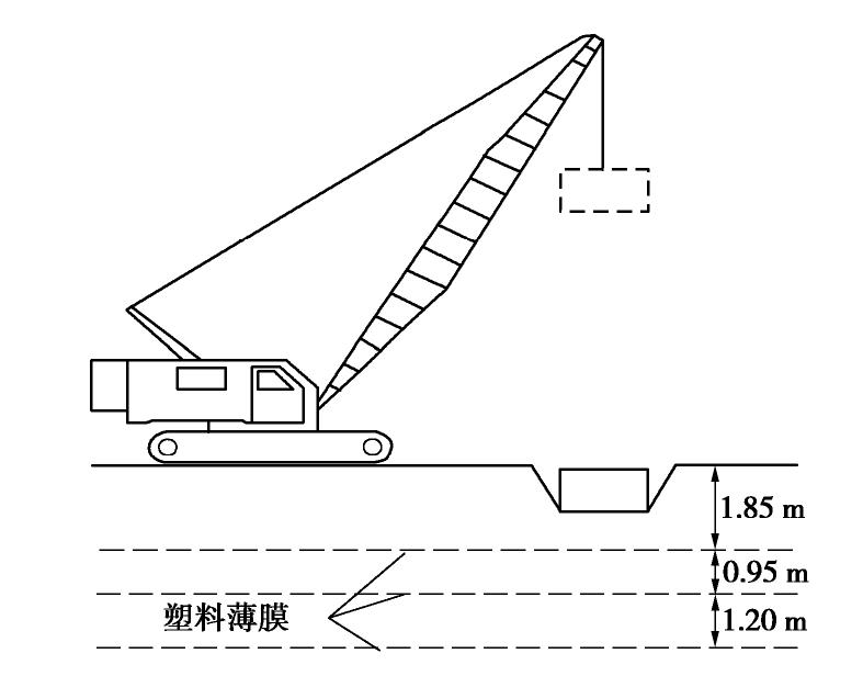
![]()
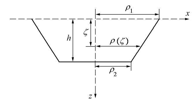
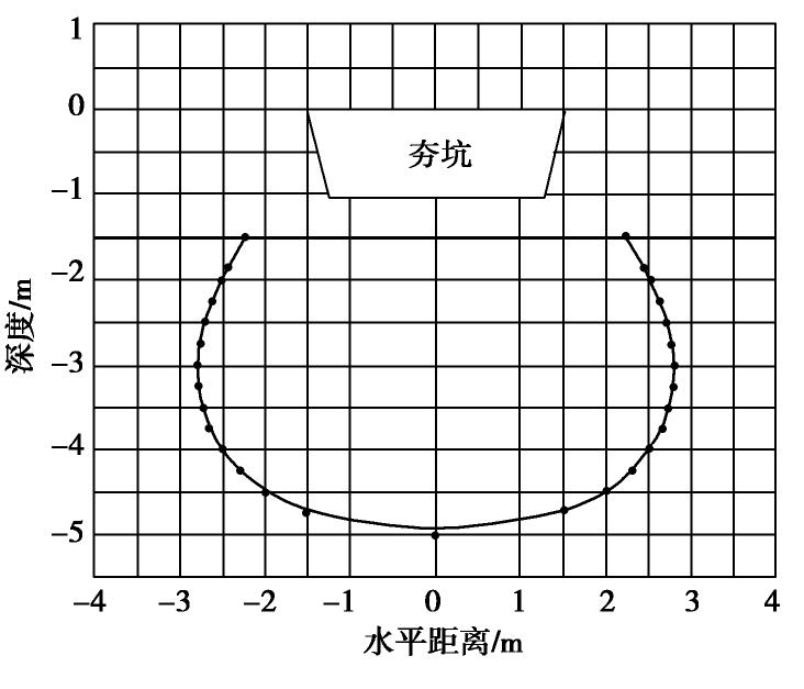
图 2 强夯过程中圆形夯锤产生的夯坑横截面示意
Figure 2. Cross section of ramming pit produced by circular rammer during dynamic compaction
![]()
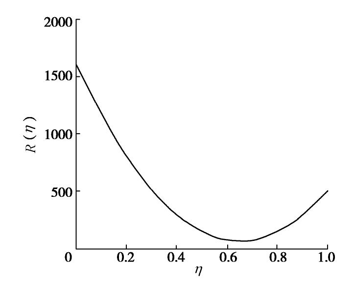
图 6 压缩系数η与最小方差
R(η) 之间的关系Figure 6. Relationship between compression coefficient and minimum variance
![]()
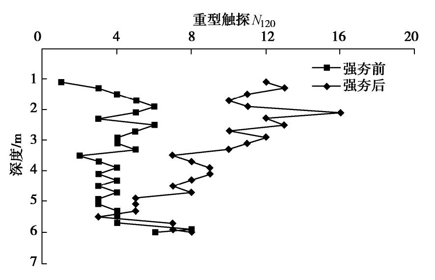
图 7 承德机场试验场地重型触探强夯前后对比
Figure 7. Comparison of heavy penetration dynamic compaction before and after test site in Chengde Airport
![]()
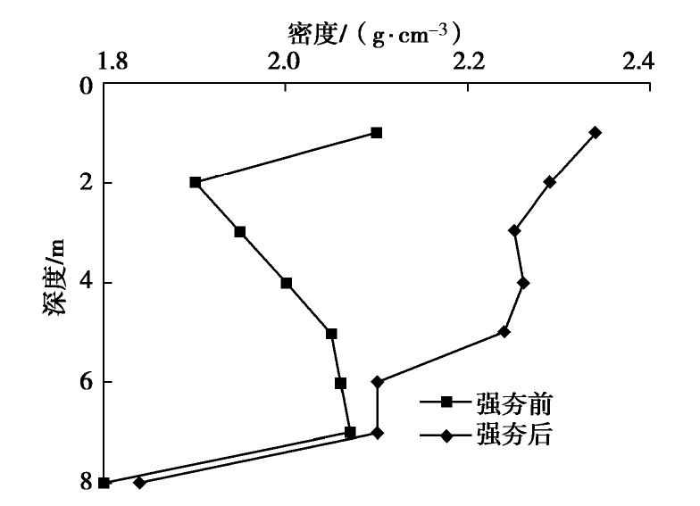
图 8 承德机场试验场地密度试验强夯前后对比
Figure 8. Comparison of density tests before and after dynamic compaction in test site in Chengde Airport
![]()
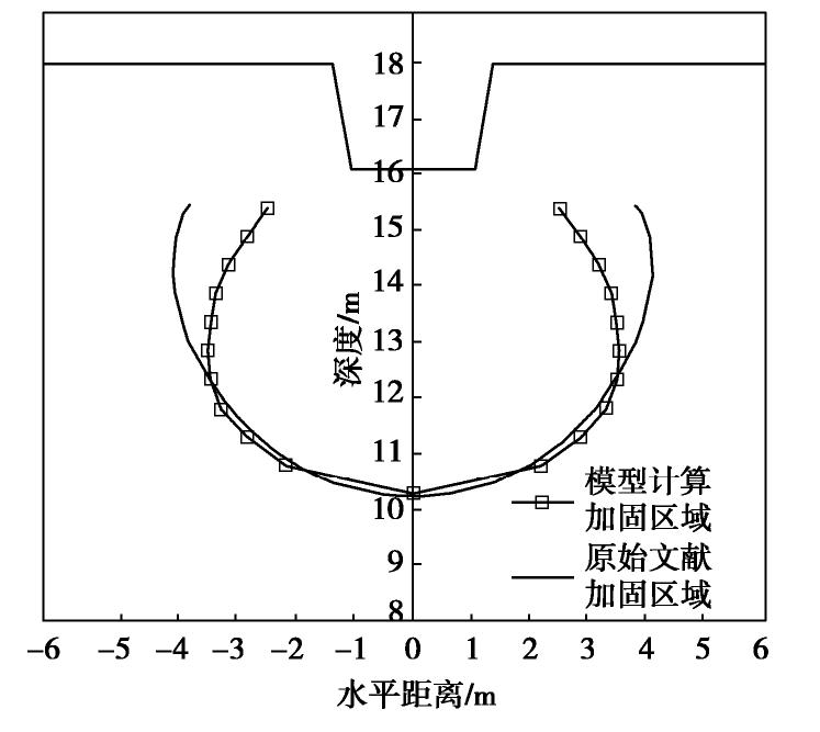
图 9 根据临界沉降量确定的强夯加固边界示意图(线内区域为内部沉降量大于0.04 m的区域)
Figure 9. Schematic diagram of dynamic consolidation boundary determined by critical settlement
![]()
![]()
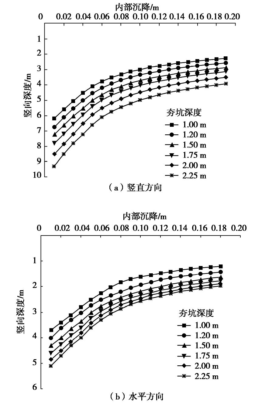
图 11 内部沉降量随夯坑深度的变化规律
Figure 11. Variation rules of internal settlement with depth of tamping pit
表 1 强夯引起位移量对比
Table 1 Comparison of displacements caused by dynamic compaction
(cm) 深度/m 结果 水平距离/m 0 1 2 3 4 5 1.86 计算值 42.00 29.27 9.62 1.59 0.16 0.00 观测值 25.50 20.50 10.00 5.00 0.00 0.00 修正值 27.30 19.03 6.25 1.03 0.10 0.00 2.80 计算值 18.80 15.90 9.69 4.29 1.40 0.35 观测值 15.50 15.50 8.00 3.00 1.00 0.00 修正值 12.22 10.34 6.30 2.79 0.90 0.23 4.00 计算值 8.88 8.22 6.50 4.41 2.57 1.29 观测值 6.00 6.00 4.00 2.50 1.50 0.00 修正值 5.80 5.40 4.20 2.90 1.67 0.84  下载: 导出CSV
表 2 强夯工程参数
Table 2 Parameters of dynamic compaction project
夯锤半径/m 夯锤质量/t 抬升高度/m 弹性模量/MPa 泊松比 ν 夯坑深度/m η 1.2 20 20 4 0.25 1.2 0.65
下载: 导出CSV
-
[1] ZEKKOS D, TSITSAS G, DIMITRIADI V, et al. Dynamic compaction of collapsible soils-case study from a motorway project in Romania[C]//XVI Ecsmge Geotechnical Engineering for Infrastructure and Development. 2015.
[2] WU Shuai-feng, WEI Ying-qi, ZHANG Yin-qiu, et al. Dynamic compaction of a thick soil-stone fill: dynamic response and strengthening mechanisms[J]. Soil Dynamics and Earthquake Engineering, 2020, 129: 105944. doi: 10.1016/j.soildyn.2019.105944
[3] ROLLINS K M, KIM J. Dynamic compaction of collapsible soils based on U.S. case histories[J]. Journal of Geotechnical and Geoenvironmental Engineering, 2010, 136(9): 1178-1186. doi: 10.1061/(ASCE)GT.1943-5606.0000331
[4] DU J F, WU S F, HOU S, et al. Deformation analysis of granular soils under dynamic compaction based on stochastic medium theory[J]. Mathematical Problems in Engineering, 2019(1): 1-10. doi: 10.1155/2019/6076013.
[5] MAYNE P W, JONES S J. Impact stresses during dynamic Compaction[J]. Journal of Geotechnical Engineering, 1983, 109(10): 1342-1346. doi: 10.1061/(ASCE)0733-9410(1983)109:10(1342)
[6] MENARD L, BROISE Y. Theoretical and practical aspects of dynamic consolidation[J]. Géotechnique, 1975, 25(1): 3-18. doi: 10.1680/geot.1975.25.1.3
[7] DURGUNOGLU H T, VARAKSIN S, BRIET S, et al. A case study on soil improvement with heavy dynamic compaction[C]//Proceedings of the 13th European Conference on Soil Mechanics and Geotechnical Engineering, 2003, Prague.
[8] MAYNE P W, JONES J S, DUMAS J C. Ground response to dynamic compaction[J]. Journal of Geotechnical Engineering, 1984, 110(6): 757-774. doi: 10.1061/(ASCE)0733-9410(1984)110:6(757)
[9] CHOW Y K, YONG D M, YONG K Y, et al. Dynamic compaction analysis[J]. Journal of Geotechnical Engineering, 1992, 118(8): 1141-1157. doi: 10.1061/(ASCE)0733-9410(1992)118:8(1141)
[10] POURJENABI M, GHANBARI E, HAMIDI A. Numerical modeling of dynamic compaction in dry sand using different constitutive models//4th ECCOMAS Thematic Conference on Computational Methods in Structural Dynamics and Earthquake Engineering, 2013. Kos Island.
[11] LITWINISZYN J. The theories and model research of movements of ground masses[C]//Proceedings of the European Congress Ground Movement. Leeds, 1957: 203-209.
[12] LIU B C, WANG M C. Modeling of tunneling-induced ground surface movements using stochastic medium theory[J]. Tunnelling and Underground Space Technology, 2004, 19(2): 113-123. doi: 10.1016/j.tust.2003.07.002
[13] 姚仰平, 张北战. 基于体应变的强夯加固范围研究[J]. 岩土力学, 2016, 37(9): 2663-2671. YAO Yang-ping, Bei-zhan Z. Reinforcement range of dynamic compaction based on volumetric strain[J]. Rock and Soil Mechanics, 2016, 37(9): 2663-2671. (in Chinese)
[14] GHASSEMI A, PAK, A, SHAHIR H. A numerical tool for design of dynamic compaction treatment in dry and moist sands[J]. Iran J Sci Tech, 2009, 33(B4): 313.
-
期刊类型引用(6)
1. 许盛,杨明山,唐志勇,杨皓宇,李小兴,刘念. 察尔汗盐湖地区饱和盐渍软土地基处理. 人民长江. 2024(S2): 178-184 .  百度学术
百度学术
2. 何鸿烈,杨扬,王志壮,司宁强,李生泽. 戈壁料高填方强夯补强应用研究. 建筑施工. 2023(03): 534-537 . 百度学术
3. 张学军. 强夯压实技术在路基补强施工的应用及优化. 建筑机械. 2023(07): 61-66+70 . 百度学术
4. 赵延林,龚雨林,张子煜. 深厚换填砂土地基强夯有效加固深度的影响因素. 黑龙江科技大学学报. 2023(05): 710-717 . 百度学术
5. 刘文俊,李岳,蔡靖,戴轩,水伟厚,董炳寅. 基于强夯应力波传播模型的夯击参数研究. 岩土力学. 2023(S1): 427-435 . 百度学术
6. 秦劭杰,戎晓宁,张路银,彭梦凯,董炳寅. 特殊场地强夯振动监测及隔振效果研究. 地基处理. 2023(S2): 84-90 . 百度学术
其他类型引用(7)


计量
- 文章访问数: 167
- HTML全文浏览量: 31
- PDF下载量: 95
- 被引次数: 13